Ng-Machine learning 课程笔记 
约 4976 个字 306 行代码 18 张图片 预计阅读时间 29 分钟
- @start 2025.3.9
- @end 2025.3.15
- 相关资源
- 我采用的方式是课程仓库 + vscode jupyter notebook plugin
- 放个正版课链接:https://www.coursera.org/specializations/machine-learning-introduction
0 什么是机器学习 
- 机器学习
- 监督学习 (supervised learning)
- 无监督学习 (unsupervised learning)
监督学习 
- 监督学习
- 回归 (regression): 通过输入预测一个连续值 ( 结果有无限多个可能 )
- 分类 (classification): 通过输入预测一个离散值 ( 从有限的可能中选择 )
- 总结:投喂的数据集有标签,让机器从中学习映射关系
无监督学习 
- 投喂的数据集没有标签,机器靠数据的特征分析模式,发现隐藏的结构,不会像监督学习产生预测值。比如投喂一些动物图片,机器根据图片特征把这些图片分成几类 ( 聚类算法 -clustering)。
- 另外的算法还有降维 (PCA)、异常检测等
1 线性回归 
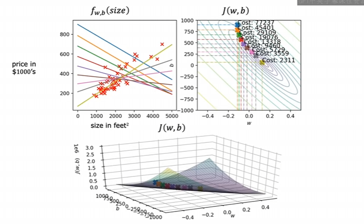
- 建立直觉:线性回归通过找出输入和输出之间的最佳直线关系来进行预测。它假设输入和输出有线性关系,先随机初始化一个线性关系,通过某种方式不断调整参数来最小化误差。
1.1 成本函数 
- 引入这个函数的目的:用于衡量模型预测的好坏
1.2 梯度下降 
- 本节讨论的实际是批量梯度下降 ("Batch" gradient descent)
- 计算从 \(j\) 值高点到 \(j\) 值低点所走的最优路径
- 下面是求偏导的结果
- 越接近 \(j(w, b)\) 的最小值,梯度下降越慢
学习率 (learing rate) 
- 如果 \(\alpha\) 过小,所需的调整次数会增加
- 如果 \(\alpha\) 过大,梯度下降可能无法收敛
可能存在的问题 
- 局部最小不是全局最小
拟合过程 
1.3 梯度下降代码实现 
import math, copy
import numpy as np
import matplotlib.pyplot as plt
plt.style.use('./deeplearning.mplstyle')
from lab_utils_uni import plt_house_x, plt_contour_wgrad, plt_divergence, plt_gradients

# Load our data set
x_train = np.array([1.0, 2.0])   # features
y_train = np.array([300.0, 500.0])   #target value

#Function to calculate the cost
def compute_cost(x, y, w, b):

    m = x.shape[0]
    cost = 0

    for i in range(m):
        f_wb = w * x[i] + b
        cost = cost + (f_wb - y[i])**2
    total_cost = 1 / (2 * m) * cost

    return total_cost

def compute_gradient(x, y, w, b):
    # Number of training examples
    m = x.shape[0]
    dj_dw = 0
    dj_db = 0

    for i in range(m):
        f_wb = w * x[i] + b
        dj_dw_i = (f_wb - y[i]) * x[i]
        dj_db_i = f_wb - y[i]
        dj_db += dj_db_i
        dj_dw += dj_dw_i
    dj_dw = dj_dw / m
    dj_db = dj_db / m

    return dj_dw, dj_db


def gradient_descent(x, y, w_in, b_in, alpha, num_iters, cost_function, gradient_function):
    w = copy.deepcopy(w_in) # avoid modifying global w_in
    # An array to store cost J and w's at each iteration primarily for graphing later
    J_history = []
    p_history = []
    b = b_in
    w = w_in

    for i in range(num_iters):
        # Calculate the gradient and update the parameters using gradient_function
        dj_dw, dj_db = gradient_function(x, y, w , b)

        # Update Parameters using equation (3) above
        b = b - alpha * dj_db
        w = w - alpha * dj_dw

        # Save cost J at each iteration
        if i<100000:      # prevent resource exhaustion
            J_history.append( cost_function(x, y, w , b))
            p_history.append([w,b])
        # Print cost every at intervals 10 times or as many iterations if < 10
        if i% math.ceil(num_iters/10) == 0:
            print(f"Iteration {i:4}: Cost {J_history[-1]:0.2e} ",
                  f"dj_dw: {dj_dw: 0.3e}, dj_db: {dj_db: 0.3e}  ",
                  f"w: {w: 0.3e}, b:{b: 0.5e}")

    return w, b, J_history, p_history #return w and J,w history for graphing

# initialize parameters
w_init = 0
b_init = 0
# some gradient descent settings
iterations = 10000
tmp_alpha = 1.0e-2
# run gradient descent
w_final, b_final, J_hist, p_hist = gradient_descent(x_train ,y_train, w_init, b_init, tmp_alpha,
                                                    iterations, compute_cost, compute_gradient)
2 多元线性回归 
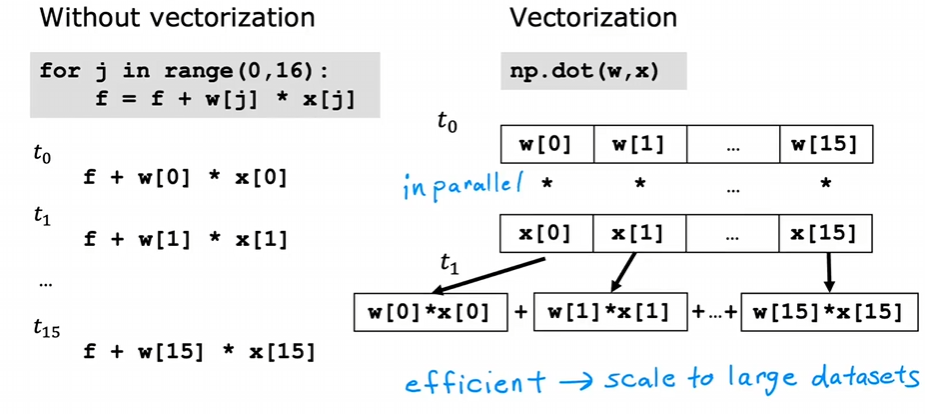
2.1 向量化 
- 原方法
- 向量化
- 原理
2.2 多元梯度下降 
2.3 多元梯度下降代码实现 
def compute_cost(X, y, w, b):
    m = X.shape[0]
    cost = 0.0
    for i in range(m):
        f_wb_i = np.dot(X[i], w) + b           #(n,)(n,) = scalar (see np.dot)
        cost = cost + (f_wb_i - y[i])**2       #scalar
    cost = cost / (2 * m)                      #scalar
    return cost

def compute_gradient(X, y, w, b):
    m,n = X.shape           #(number of examples, number of features)
    dj_dw = np.zeros((n,))
    dj_db = 0.

    for i in range(m):
        err = (np.dot(X[i], w) + b) - y[i]
        for j in range(n):
            dj_dw[j] = dj_dw[j] + err * X[i, j]
        dj_db = dj_db + err
    dj_dw = dj_dw / m
    dj_db = dj_db / m

    return dj_db, dj_dw

def gradient_descent(X, y, w_in, b_in, cost_function,
    # An array to store cost J and w's at each iteration primarily for graphing later
    J_history = []
    w = copy.deepcopy(w_in)  #avoid modifying global w within function
    b = b_in

    for i in range(num_iters):

        # Calculate the gradient and update the parameters
        dj_db,dj_dw = gradient_function(X, y, w, b)   ##None

        # Update Parameters using w, b, alpha and gradient
        w = w - alpha * dj_dw               ##None
        b = b - alpha * dj_db               ##None

        # Save cost J at each iteration
        if i<100000:      # prevent resource exhaustion
            J_history.append( cost_function(X, y, w, b))

        # Print cost every at intervals 10 times or as many iterations if < 10
        if i% math.ceil(num_iters / 10) == 0:
            print(f"Iteration {i:4d}: Cost {J_history[-1]:8.2f}   ")

    return w, b, J_history #return final w,b and J history for graphing

# initialize parameters
X_train = np.array([[2104, 5, 1, 45], [1416, 3, 2, 40], [852, 2, 1, 35]])
y_train = np.array([460, 232, 178])
initial_w = np.zeros_like(w_init)
initial_b = 0.
# some gradient descent settings
iterations = 1000
alpha = 5.0e-7
# run gradient descent
w_final, b_final, J_hist = gradient_descent(X_train, y_train, initial_w, initial_b,
                                                    compute_cost, compute_gradient,
                                                    alpha, iterations)
2.4 特征缩放 
- 目的是加速梯度下降的收敛
- 由于不同特征的数量级可能会有差异,导致对应的 \(w_{i}\) 权重更高,后果是梯度下降走 Z 字。
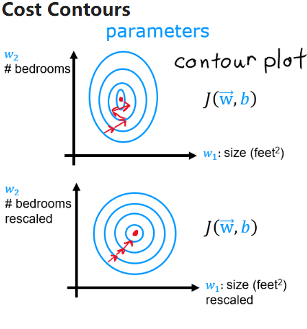
- 均值归一化
- z-score 归一化
- 归一化,所有要素平均值为 0,标准差为 1
2.5 z-score 归一化代码实现 
def zscore_normalize_features(X):
    """
    computes  X, zcore normalized by column

    Args:
      X (ndarray (m,n))     : input data, m examples, n features

    Returns:
      X_norm (ndarray (m,n)): input normalized by column
      mu (ndarray (n,))     : mean of each feature
      sigma (ndarray (n,))  : standard deviation of each feature
    """
    # find the mean of each column/feature
    mu     = np.mean(X, axis=0)                 # mu will have shape (n,)
    # find the standard deviation of each column/feature
    sigma  = np.std(X, axis=0)                  # sigma will have shape (n,)
    # element-wise, subtract mu for that column from each example, divide by std for that column
    X_norm = (X - mu) / sigma

    return (X_norm, mu, sigma)
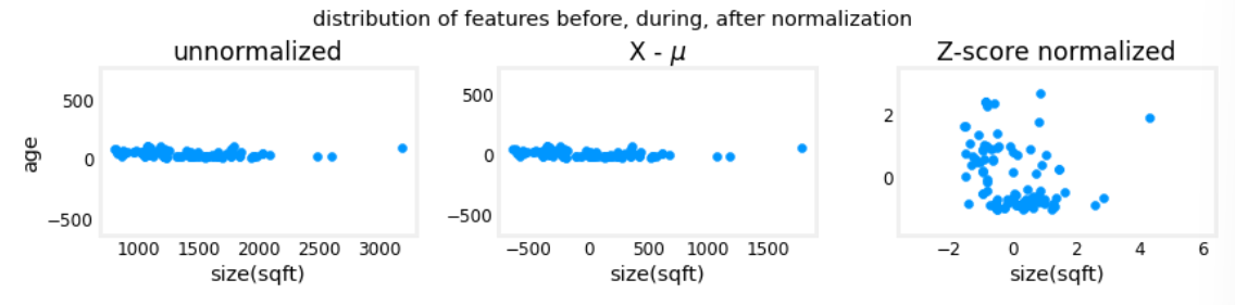
- axis=0 表示逐列求均值,axis=1 表示逐行求均值
- 下面是三种特征缩放的对比图
进行预测
#predict target using normalized features
m = X_norm.shape[0]
yp = np.zeros(m)
for i in range(m):
    yp[i] = np.dot(X_norm[i], w_norm) + b_norm

    # plot predictions and targets versus original features
fig,ax=plt.subplots(1,4,figsize=(12, 3),sharey=True)
for i in range(len(ax)):
    ax[i].scatter(X_train[:,i],y_train, label = 'target')
    ax[i].set_xlabel(X_features[i])
    ax[i].scatter(X_train[:,i],yp,color=dlc["dlorange"], label = 'predict')
ax[0].set_ylabel("Price"); ax[0].legend();
fig.suptitle("target versus prediction using z-score normalized model")
plt.show()
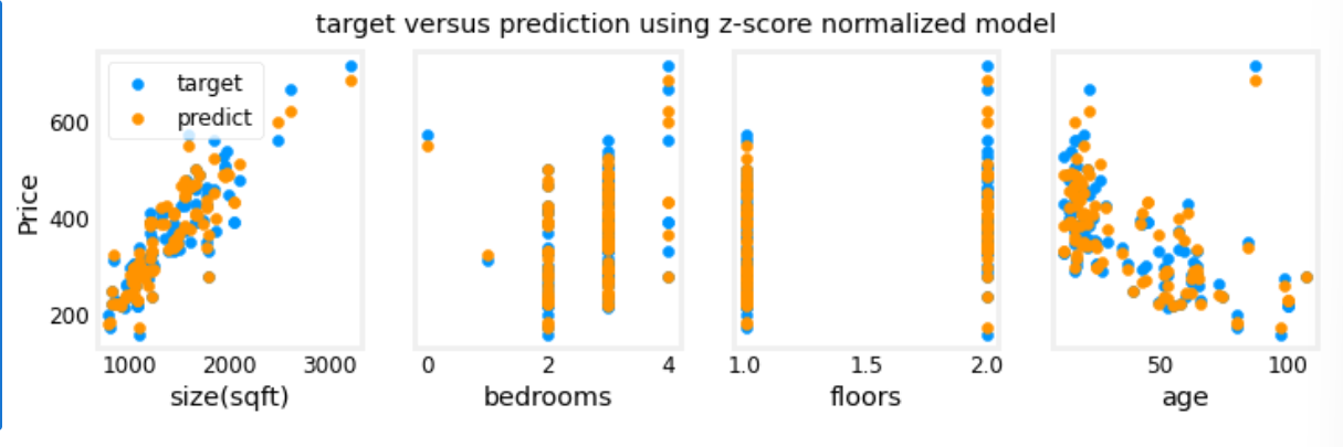
- 用于预测的 input 也必须标准化
怎么选择合适的学习率 
- 尝试并观察参数变化
2.6 特征工程和多项式回归 
- 特征工程:从原始数据中提取、转换或创建更有意义的特征,以提高机器学习模型的表现,能够提高预测准确性
- 如发现 \(wx+b\) 拟合效果不好,创建一个特征 \(x^2\) , 尝试用 \(w_{0}x_{0}+w_{1}x_{1}^2\)
- 没有进行梯度下降之前就可以使用替代视图进行拟合效果分析
# create target data
x = np.arange(0, 20, 1)
y = x**2

# engineer features .
X = np.c_[x, x**2, x**3]   #<-- added engineered feature
X_features = ['x','x^2','x^3']

fig,ax=plt.subplots(1, 3, figsize=(12, 3), sharey=True)
for i in range(len(ax)):
    ax[i].scatter(X[:,i],y)
    ax[i].set_xlabel(X_features[i])
ax[0].set_ylabel("y")
plt.show()
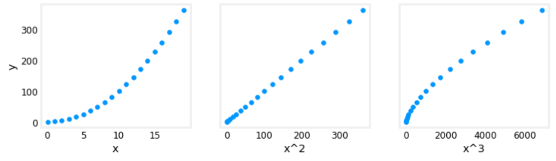
- 一个问题是 \(x,x^2,x^3\) 的尺度可能会有较大差异,可以使用 z-score 归一化来解决
x = np.arange(0,20,1)
y = x**2

X = np.c_[x, x**2, x**3]
X = zscore_normalize_features(X)

model_w, model_b = run_gradient_descent_feng(X, y, iterations=100000, alpha=1e-1)
- 可以应用特征工程对相对复杂的函数建模,泰勒已经告诉了我们这个结论
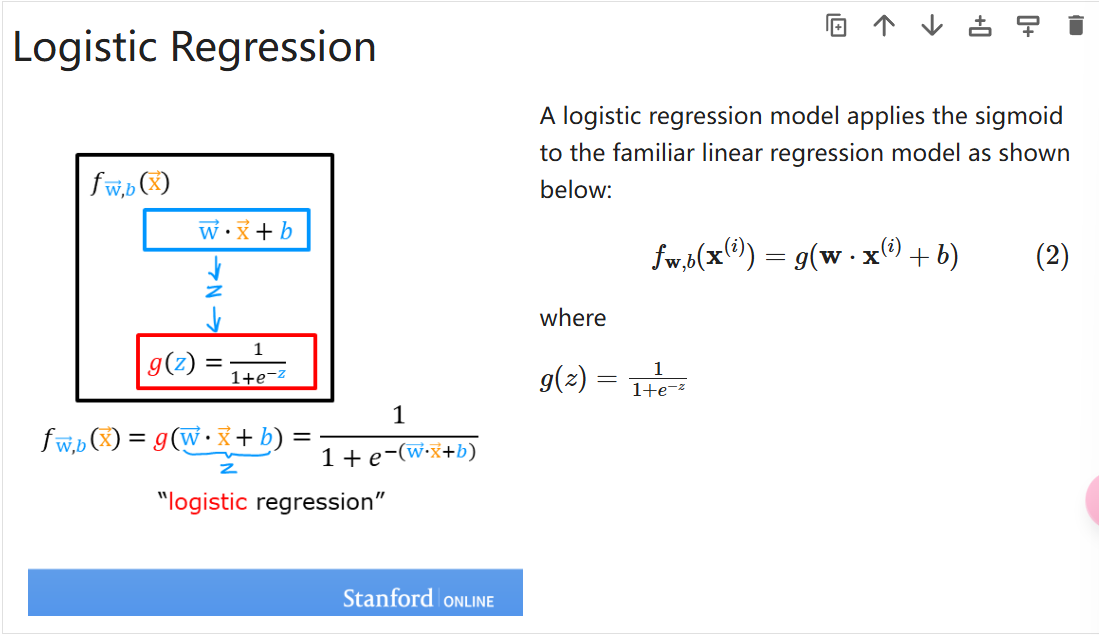
3 逻辑回归 
- 一种用于二分类的算法
- 原先的线性方程不能很好地拟合二分类的图像
- 于是进行了巧妙的映射,如下
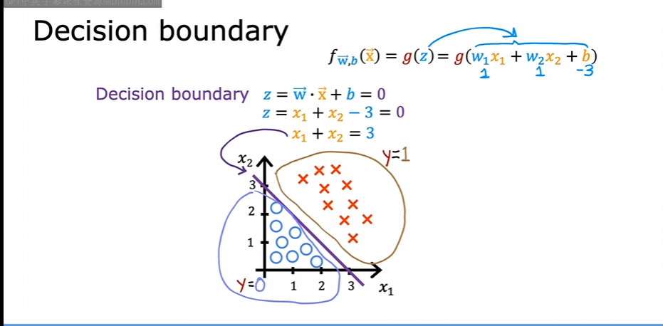
3.1 决策边界 
在逻辑回归中,我们使用 Sigmoid 函数 计算概率:
一般当 \(g(z) = \frac{1}{1+e^{-z}}>0.5\) 时,我们认为 y = 1, 而这个点恰好对应 \(\vec{w}\vec{x}+b=0\)
3.2 逻辑回归的成本函数 
如果还是使用线性回归的成本函数,得到的曲线有多个局部最小值。所以需要另外定义一个成本函数。
- 逻辑回归的损失函数如下,只针对一个样本
也可以简写为
合理之处在于如果预测值接近正确类别损失较小,如果预测值接近错误类别损失较大,同时连续且可微,便于梯度下降优化
- 成本函数如下
- 代码实现
def compute_cost_logistic(X, y, w, b):
    m = X.shape[0]
    cost = 0.0
    for i in range(m):
        z_i = np.dot(X[i],w) + b
        f_wb_i = sigmoid(z_i)
        cost +=  -y[i]*np.log(f_wb_i) - (1-y[i])*np.log(1-f_wb_i)

    cost = cost / m
    return cost
3.3 将梯度下降应用到逻辑回归 
逻辑回归的梯度下降仍然满足下式
- 代码实现
def compute_gradient_logistic(X, y, w, b):

    m,n = X.shape
    dj_dw = np.zeros((n,))                           #(n,)
    dj_db = 0.

    for i in range(m):
        f_wb_i = sigmoid(np.dot(X[i],w) + b)          #(n,)(n,)=scalar
        err_i  = f_wb_i  - y[i]                       #scalar
        for j in range(n):
            dj_dw[j] = dj_dw[j] + err_i * X[i,j]      #scalar
        dj_db = dj_db + err_i
    dj_dw = dj_dw/m                                   #(n,)
    dj_db = dj_db/m                                   #scalar

    return dj_db, dj_dw

def gradient_descent(X, y, w_in, b_in, alpha, num_iters):
    # An array to store cost J and w's at each iteration primarily for graphing later
    J_history = []
    w = copy.deepcopy(w_in)  #avoid modifying global w within function
    b = b_in

    for i in range(num_iters):
        # Calculate the gradient and update the parameters
        dj_db, dj_dw = compute_gradient_logistic(X, y, w, b)

        # Update Parameters using w, b, alpha and gradient
        w = w - alpha * dj_dw
        b = b - alpha * dj_db

        # Save cost J at each iteration
        if i<100000:      # prevent resource exhaustion
            J_history.append( compute_cost_logistic(X, y, w, b) )

        # Print cost every at intervals 10 times or as many iterations if < 10
        if i% math.ceil(num_iters / 10) == 0:
            print(f"Iteration {i:4d}: Cost {J_history[-1]}   ")

    return w, b, J_history         #return final w,b and J history for graphing
3.4 过拟合 
对给出的样本拟合效果很好但是预测效果不佳
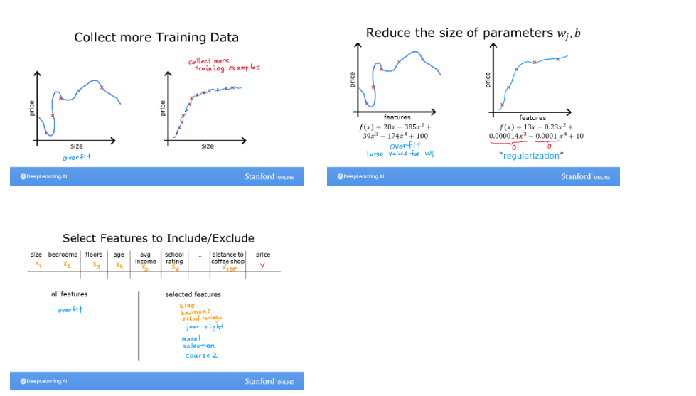
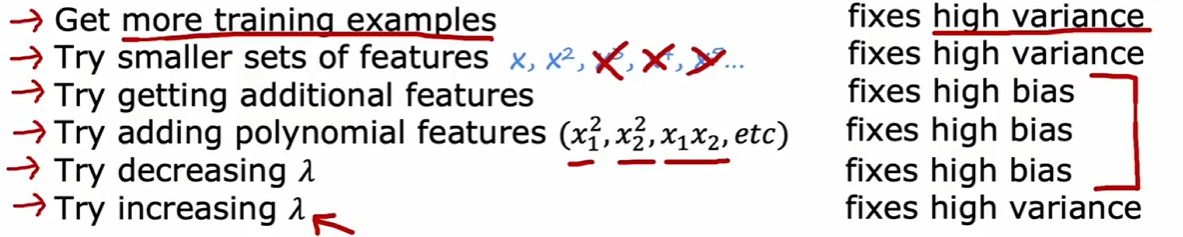
3.5 解决过拟合 
- 更多的训练数据
- 减少特征数量
- 正则化
正则化 
- 对于高阶的特征项,我们通常希望它们的系数较小,以减少模型复杂度,防止过拟合
对此我们需要更改成本函数表达式
对于线性回归
对于逻辑回归
梯度下降实现相同
不展示实现了,多了几项而已
4 神经网络 
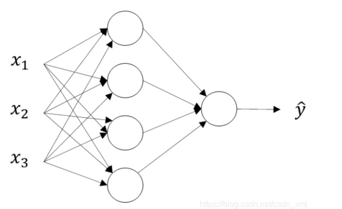
- 建立直觉:大概意思就是,每一个神经元的输出作为下一个神经元的输入,最后一个神经元的输出就是预测结果 . 每一个神经元都有自己的 w 和 b, 开始时随机初始化每一组 w 和 b 的值,通过迭代训练调整 w 和 b 使成本最小。如果神经网络很复杂,那么 w 和 b 的变化往往是人类不能理解的。
4.1 流程 
- 前向传播
- 计算损失
- 反向传播更新参数
- 迭代训练
4.2 多类别 
放一个代码实现:
# explanation
classes = 4 # number of classes
m = 100 # number of samples
centers = [[-5, 2], [-2, -2], [1, 2], [5, -2]] # centers of the clusters
std = 1.0 # standard deviation of the clusters
X_train, y_train = make_blobs(n_samples=m, centers=centers, cluster_std=std,random_state=30) # generate training data

tf.random.set_seed(1234)  # Set the seed for reproducibility
model = Sequential(
    [
        Dense(2, activation = 'relu',   name = "L1"),
        Dense(4, activation = 'linear', name = "L2")
    ]
)
# Compile the model
model.compile(
    loss=tf.keras.losses.SparseCategoricalCrossentropy(from_logits=True), # SparseCategoricalCrossentropy is used because the labels are integers
    optimizer=tf.keras.optimizers.Adam(0.01), # use Adom optimizer with learning rate of 0.01
)

model.fit(
    X_train,y_train,
    epochs=200
)
4.3 其它激活函数 
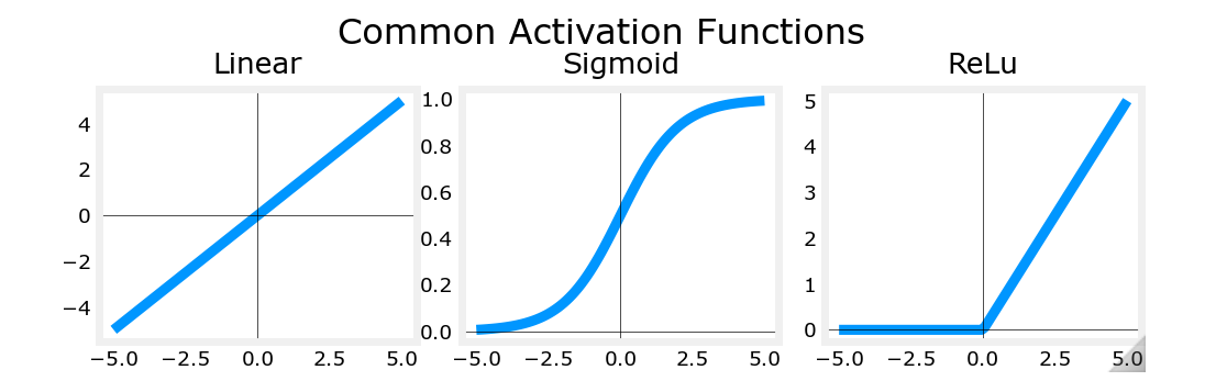
ReLU
ReLU 的合理性 
- 避免不必要的输出,提高训练效率
- 解决梯度消失的问题
softmax
- softmax 的损失函数
- softmax 的成本函数
- Tensorflow 实现稀疏分类交叉熵损失的两种方法:
way 1
model = Sequential(
    [
        Dense(25, activation = 'relu'),
        Dense(15, activation = 'relu'),
        Dense(4, activation = 'softmax')    # < softmax activation here
    ]
)
model.compile(
    loss=tf.keras.losses.SparseCategoricalCrossentropy(),
    optimizer=tf.keras.optimizers.Adam(0.001),
)

model.fit(
    X_train,y_train,
    epochs=10
)
way 2
preferred_model = Sequential(
    [
        Dense(25, activation = 'relu'),
        Dense(15, activation = 'relu'),
        Dense(4, activation = 'linear')   #<-- Note
    ]
)
preferred_model.compile(
    loss=tf.keras.losses.SparseCategoricalCrossentropy(from_logits=True),  #<-- Note
    optimizer=tf.keras.optimizers.Adam(0.001),
)

preferred_model.fit(
    X_train,y_train,
    epochs=10
)
- 第二种方法优于第一种方法
- 第二种方法将 softmax 操作包含在损失计算中,这个情况下,计算机会采取更好的方法进行计算从而得到更准确的结果
- 课程中的例子:python 中计算 \(1+\frac{1}{1000000}-(1-\frac{1}{1000000})\) 和 \(\frac{1}{1000000}+\frac{1}{1000000}\) 时得到的结果是不一样的
稀疏分类交叉熵和分类交叉熵 
- SparseCategorialCrossentropy:期望目标是与索引对应的整数。例如,如果有 10 个可能的目标值,则 y 将介于 0 和 9 之间。
- CategoricalCrossEntropy:预期示例的目标值为 one-hot 编码,其中目标索引的值为 1,而其他 N-1 个条目为零。具有 10 个潜在目标值的示例,其中目标为 2,则为 [0,0,1,0,0,0,0,0,0,0]。
5 模型评估 
5.1 概念汇总 
- 数据集
- 训练集 (training set):用于模型训练
- 交叉验证集 (dev set):训练过程中用于模型选择和超参数调优,帮助确定最佳的模型配置
- 测试集 (test set):用于评估模型在新数据上的表现,反应模型的泛化能力,测试集的数据在训练过程中不可见
- 如果采用测试集进行模型选择会导致实际误差大于泛化误差,因为测试集实际上介入了模型选择的过程。
- 误差
- 实际误差:模型拟合数据的 " 现状 " 反映
- 泛化误差:模型在所有可能的新样本上的预期误差
- 基准性能水平:为衡量模型水平设定的参考标准,比如人类预测的准确率
- 正则化
- 目的:通过增加正则化项来防止模型过拟合
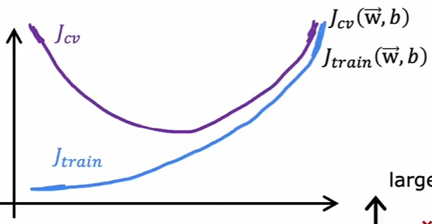
- 偏差与方差:
- 高偏差:模型过于简单,不能捕捉数据规律
- 高方差:模型过于复杂,对训练数据过度拟合,在新数据上表现过差
一般来说,验证集的成本函数和训练集的成本函数有如下关系
5.2 偏差方差和神经网络 
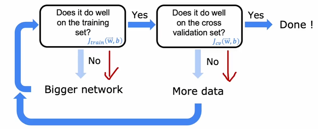
解决偏差和方差问题的策略如下
理论上,采用更加庞大的神经网络时,只要恰当地正则化,那么至少拥有和小型神经网络相仿的拟合结果
5.3 数据扩充 
- 错误分析:
- 数据扩充:当数据量有限时采用数据扩充来获取新数据
- 数据增强:改造现有数据,生成新的样本,如图像识别中对已有图像进行旋转,裁剪,扭曲得到新图像
- 数据合成:利用算法合成新的数据
- 迁移学习:当没有足够数据时,利用相似的已经经过预训练的模型得到相对合理的 w 和 b 作为初始值而不是采用随机值
- 只训练最后一层:当数据量不足时
- 全部训练:在预训练的基础上,对所有层进行调整
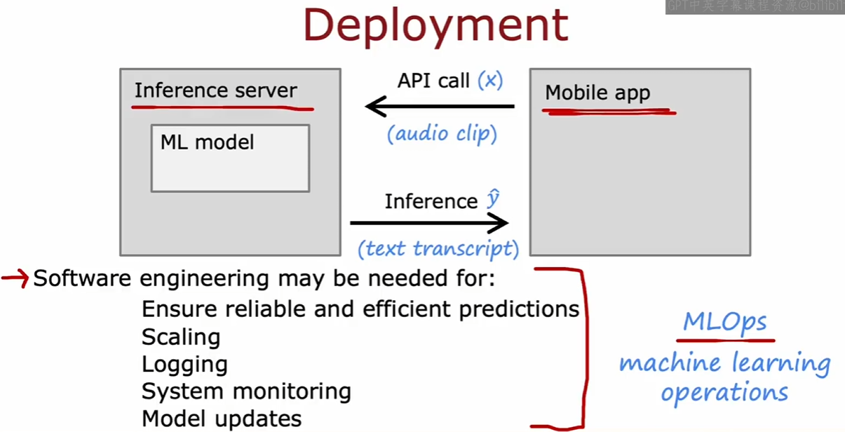
5.4 机器学习项目的完整周期 
决定项目内容和你要解决的问题 -> 收集数据 -> 训练模型 -> 模型评估考虑优化训练方式 -> 部署,监视,维护模型
5.5 处理倾斜数据集与评价指标 
- 倾斜数据集:数据集类别分布极不平衡,比如预测罕见病
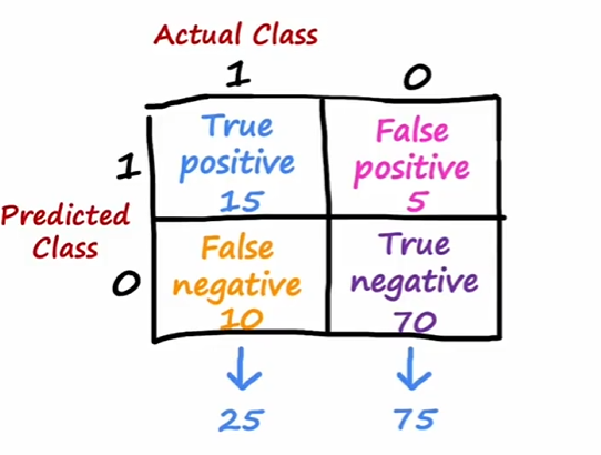
- 评价指标
- 精确率 : true pos / pre pos
- 召回率 : true pos /act pos ( 能在患病群体中甄别出多少人 )
- F1-score: 精确率和召回率的调和平均 \(\frac{PR}{P+R}\)
下面是对阴阳性的定义
6 决策树 
- 建立直觉:拿到一份数据集后,决策树通过一系列的 条件判断(例如:某特征是否大于某个值)将数据划分为不同的子集,直到每个子集的样本满足某个条件 ( 此时你认为它分决策得不错 )。最终的结果是一个树形结构,其中每个叶子节点表示预测结果。决策树通过递归的方式构建。
- 构建一棵决策树的流程
- 数据准备
- 选择分裂标准
- 超参数调优
- 独热编码的分类特征:将每一个分类的值转换为二进制向量。
6.1 以信息增益作为分裂标准示例 
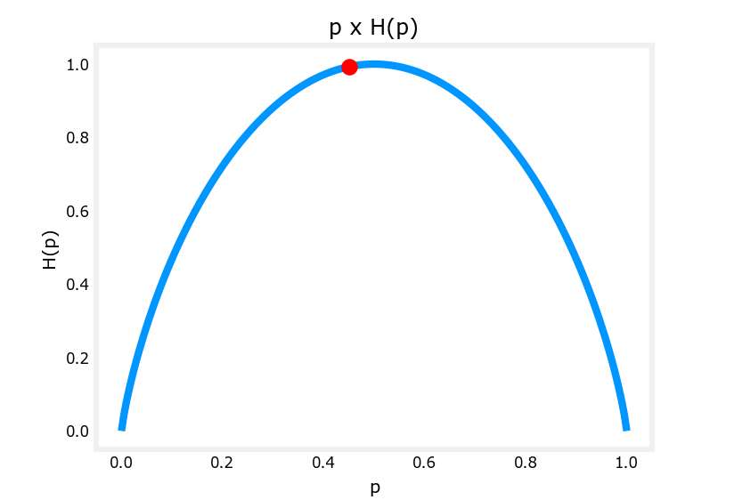
信息增益 ( 熵减程度 ):
6.2 回归树 
- 和决策树对比
- 回归树预测连续数值
- 决策树预测离散的标签
- 回归树使用均方误差作为分裂标准
- 决策树通常使用信息增益或基尼系数作为分裂标准
6.3 随机森林 
- 单棵决策树鲁棒性差的原因
- 对数据集的细微变化很敏感 , 有时如果只是新增加了一个数据 , 可能会导致整棵树的结构被重构 ( 如果恰好改变了根节点的特征 )
- 随机森林机制:随机选取数据集的子集构建树集成,多棵树投票决定最终结果
- 随机森林机制的合理性 :
- 树之间相对独立 , 而 VB 可能会导致所有树共享相似的数据字集 , 从而在相似的特征做决策 , 导致泛化能力下降
6.4 XG Boost
构建了一棵决策树后 , 第二棵决策树的数据集不再随机 , 而是更倾向于选择第一棵决策树分类错误的数据 ( 刻意练习 )
7 选择哪种模型 ? 
- 决策树 ( 树集成 )
- 适用于结构化数据
- 规模小的决策树容易被人类理解
- 神经网络
- 适用于任意类型的数据
- 训练周期长
- 适用于迁移学习
- 容易组合使用
8 K-Means
- 建立直觉:K-Means 是一种用聚类的算法,将数据集划分为 K 个簇,使同簇数据点更相似,不同簇的数据点差异更大。
其成本函数:
- 初始化:从数据集中随机选择 K 个点作为聚类中心,记作 \(\mu_{i}\sim\mu_{k}\)
- 迭代以下步骤:
- 对每个数据点 \(x_{i}\) 计算它到每个聚类中心的欧几里得距离,并将其分配给最近的那个
- 找到新的聚类中心
- 直到聚类中心不再更新或者达到最大迭代次数
- 改进初始化
- 进行多次随机的初始化,选择成本函数最低的那个
- elbow method
- 根据所需 ( 课程中以衣服尺码为例子 )
9 异常检测 
- 建立直觉:它通过分析数据分布、特征之间的关系或使用模型学习正常数据的模式,进而发现不符合这些模式的异常值
- 计算均值和方差
- 使用高斯分布建模数据
- 计算概率
- 选择合理的阈值
- 在验证集上选择 F1-score 最优的阈值
9.1 调整 
有时候数据不符合高斯分布,那么需要对数据进行变换如 \(x_{i}\to\ln{x_{i}}\)
10 协同过滤 
以电影为例子
\(n_{m}\) 部电影, \(n_{u}\) 个用户, \(Y_{ij}\) 表示用户 j 对电影 i 的评分
评分指示矩阵 \(R_{ij}\) 如果用户 j 评价了电影 i 则值为 1 否则为 0
- 成本函数
- 对成本函数梯度下降更新参数来训练模型 ( 课程中采用 tensorflow 库函数实现 )
- 推广到二元只需要进行 sigmoid 的复合,成本函数变换为二元交叉熵即可
- 协同过滤的局限性
- 数据稀疏时效果不好
- 冷启动问题:新加入的用户没有历史评分数据
- 归一化解决冷启动问题:
- \(\tilde{y}(i,j) = y(i,j) - \mu^{(j)}\) 其中 \(\mu^{(j)} = \frac{\sum_{i=1}^{n_m} r(i,j) y(i,j)}{\sum_{i=1}^{n_m} r(i,j)}\) 预测阶段需加回 \(\mu^{(i)}\)
11 基于内容的过滤 
- 概括:结合物品的特征和用户的特征 ( 历史偏好 ) 来推荐
-
下图清晰地展示了训练逻辑
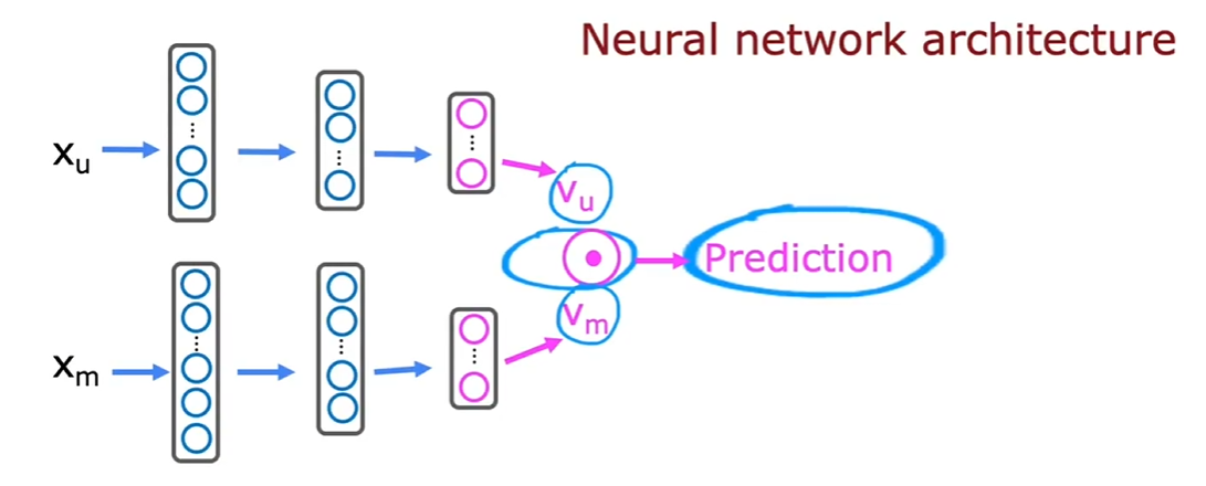
-
\(x_{u}\) 和 \(x_{m}\) 的维度不一定要相同,只需要输出的 \(v_{u}\) 和 \(v_{m}\) 维度相同
- 成本函数:
- 从大型目录中推荐 : 先检索 ( 找最相关 ) 再排序
12 强化学习 
-
建立直觉:设定某种反馈机制,不断尝试不同的动作,通过反馈结果来改进决策,从而找到最优决策
-
贝尔曼方程 (MDP 的思想 )
- 对 Lunar lander 的概括:随机初始化神经网络中的每一组 w 和 b,使降落器随机运动,存储 10000 组数据,制作成输入 - 标签对,然后训练神经网络。其中贝尔曼方程的第二项是由神经网络预测的。这种训练方法被称为 DQN 算法 (Deep Q Network)
- 在创建数据的时候采用一种更科学的方式———— \(\epsilon\) - 贪心算法:以一个小概率 ϵ 选择一个随机的动作进行探索,而以 1- \(\epsilon\) 的概率进行回报最大的探索。
- 合理性:防止了局部最优,意思是可能导致永远不会探索到某个有可能引发好结果的动作
- 一般采用逐步减小 \(\epsilon\) 的做法
关于 DNQ 的一些理解:
- 如果状态值是离散的,那么 Q 学习可以通过遍历每个状态和动作来更新 Q 的值,但是如果状态时连续的,这个过程就不可行
- 所以引入了 DNQ ,通过训练神经网络来使得输出的 Q (s, a) 尽可能最优
- 由于每次更新 Q 网络时,目标项 y 依赖于当前网络的输出 \(Q(s^{'},a^{'};w)\) ,所以成本函数的标签和预测值都在变化,可能会不稳定 ( 我也不太理解这里的不稳定 )
- 于是引入目标网络,目标网络的参数只有经过一定的步长才会更新,并且采用软更新的方式, \(w^-\leftarrow \tau w + (1 - \tau) w^-\) 这样可以使更新变得更平滑。